In this post we are going to plot candlestick charts from the stock daily quotes downloaded from Yahoo Finance using Python. Did you check our new course on Probability and Statistics For Traders? In this course we show in easy and step by step manner how you can use probability and statistics in your daily trading.
This is a purely educational posts for those who are interested in using Python for Quantitative Trading. We will be using the matplotlib library. There is a some confusion as I was consulting a book that teaches how to use Python For Finance by Yves Hilpisch. The Python code given in that book for plotting candlestick charts doesn’t work. It gives error like there is not attribute quotes_historical_yahoo and there is no attribute candlesticks. The problem with Python is that it is updated and most of the time it is not back compatible. So first we need to check the matplotlib module and its matplotlib.finance directory to check the relevant methods that are available for use.
> import matplotlib
… dir(matplotlib.finance)
…
…
… [‘Affine2D’, ‘Line2D’, ‘LineCollection’, ‘PolyCollection’, ‘Rectangle’, ‘TICKLEFT’, ‘TICKRIGHT’, ‘__builtins__’, ‘__cached__’, ‘__doc__’, ‘__file__’, ‘__loader__’, ‘__name__’, ‘__package__’, ‘__spec__’, ‘_candlestick’, ‘_check_input’, ‘_parse_yahoo_historical’, ‘_plot_day_summary’, ‘_quotes_historical_yahoo’, ‘absolute_import’, ‘cachedir’, ‘candlestick2_ochl’, ‘candlestick2_ohlc’, ‘candlestick_ochl’, ‘candlestick_ohlc’, ‘colorConverter’, ‘contextlib’, ‘date2num’, ‘datetime’, ‘division’, ‘fetch_historical_yahoo’, ‘get_cachedir’, ‘hashlib’, ‘index_bar’, ‘iterable’, ‘md5’, ‘mkdirs’, ‘np’, ‘os’, ‘parse_yahoo_historical_ochl’, ‘parse_yahoo_historical_ohlc’, ‘plot_day_summary2_ochl’, ‘plot_day_summary2_ohlc’, ‘plot_day_summary_oclh’, ‘plot_day_summary_ohlc’, ‘print_function’, ‘quotes_historical_yahoo_ochl’, ‘quotes_historical_yahoo_ohlc’, ‘six’, ‘stock_dt_ochl’, ‘stock_dt_ohlc’, ‘unicode_literals’, ‘urlopen’, ‘verbose’, ‘volume_overlay’, ‘volume_overlay2’, ‘volume_overlay3’, ‘warnings’, ‘xrange’, ‘zip’]
In the above list, you can see there is no quotes_historical_yahoo but instead there are a number of methods like _quotes_historical_yahoo, quotes_historical_yahoo_ohlc. Let’s use the method _quotes_historical_yahoo. This method is going to download the stock daily data from Yahoo Finance. We can also use pandas but the problem is the date format that matplotlib.finance module uses to draw the candlestick charts is different and in an epoch format. So we will have to use this method to download the data so that it is automatically in the proper format. We need to run this code to check it now whether this is the right method to download Dow Jones Index daily quotes data from Yahoo Finance. The ticker symbol for Dow Jones Index is ^DJI. So let’s start.
>> import matplotlib.finance as mpf
> start = (2016, 5, 1)
>>> end = (2016, 6, 30)
>>> quotes = mpf._quotes_historical_yahoo(‘^DJI’, start, end)
>>> quotes[:3]>>>
[(736086.0, 17783.779297000001, 17891.160156000002, 17912.349609000001, 17773.710938, 80100000.0), (736087.0, 17870.75, 17750.910156000002, 17870.75, 17670.880859000001, 97060000.0), (736088.0, 17735.019531000002, 17651.259765999999, 17738.060547000001, 17609.009765999999, 95020000.0)]
The above code runs and prints the first 3 quotes that were down loaded. The data is in a different format to the usual format that we are accustomed to. For example, the data download is a tuple and the date is in an epoch format unlike the date format 2016-5-1 that we had specified in the code. But this is how it is. Matplotlib needs this format to draw the candlestick charts. So let’s check this code!
#import libraries

import matplotlib.pyplot as plt

import matplotlib.finance as mpf
#import the daily stock quotes from Yahoo Finance
start = (2016, 5, 1)
end = (2016, 6, 30)
quotes = mpf._quotes_historical_yahoo(‘^DJI’, start, end)
quotes[:3]
#plot the candlestick chart
fig, ax = plt.subplots(figsize=(8, 5))
fig.subplots_adjust(bottom=0.2)
mpf.candlestick_ohlc(ax, quotes, width=0.6, colorup=’b’, colordown=’r’)
plt.grid(True)
ax.xaxis_date()
# dates on the x-axis
ax.autoscale_view()
plt.setp(plt.gca().get_xticklabels(), rotation=30)
Let’s run it on Spyder! This is the output.
>> import matplotlib.pyplot as plt
>>> import matplotlib.finance as mpf
>>>
>>> start = (2016, 5, 1)
[(736086.0, 17783.779297000001, 17891.160156000002, 17912.349609000001, 17773.710938, 80100000.0), (736087.0, 17870.75, 17750.910156000002, 17870.75, 17670.880859000001, 97060000.0), (736088.0, 17735.019531000002, 17651.259765999999, 17738.060547000001, 17609.009765999999, 95020000.0)]
>>> end = (2016, 6, 30)
>>> quotes = mpf._quotes_historical_yahoo(‘^DJI’, start, end)
>>> quotes[:3]
>>>
([<matplotlib.lines.Line2D object at 0x000001B8291D49B0>, <matplotlib.lines.Line2D object at 0x000001B8291EC0B8>, <matplotlib.lines.Line2D object at 0x000001B8291F0F60>, <matplotlib.lines.Line2D object at 0x000001B8291F6EB8>, <matplotlib.lines.Line2D object at 0x000001B8291FBFD0>, <matplotlib.lines.Line2D object at 0x000001B8293262E8>, <matplotlib.lines.Line2D object at 0x000001B82932B400>, <matplotlib.lines.Line2D object at 0x000001B829331518>, <matplotlib.lines.Line2D object at 0x000001B829337630>, <matplotlib.lines.Line2D object at 0x000001B82933E748>, <matplotlib.lines.Line2D object at 0x000001B829342860>, <matplotlib.lines.Line2D object at 0x000001B82934A978>, <matplotlib.lines.Line2D object at 0x000001B82934EA90>, <matplotlib.lines.Line2D object at 0x000001B8291871D0>, <matplotlib.lines.Line2D object at 0x000001B829198D68>, <matplotlib.lines.Line2D object at 0x000001B82918D978>, <matplotlib.lines.Line2D object at 0x000001B829353EF0>, <matplotlib.lines.Line2D object at 0x000001B829362208>, <matplotlib.lines.Line2D object at 0x000001B829368320>, <matplotlib.lines.Line2D object at 0x000001B82936D438>, <matplotlib.lines.Line2D object at 0x000001B829374550>, <matplotlib.lines.Line2D object at 0x000001B82937A668>, <matplotlib.lines.Line2D object at 0x000001B82937F780>, <matplotlib.lines.Line2D object at 0x000001B829385898>, <matplotlib.lines.Line2D object at 0x000001B82938C9B0>, <matplotlib.lines.Line2D object at 0x000001B829390AC8>, <matplotlib.lines.Line2D object at 0x000001B829396BE0>, <matplotlib.lines.Line2D object at 0x000001B82939CCF8>, <matplotlib.lines.Line2D object at 0x000001B8293A2E10>, <matplotlib.lines.Line2D object at 0x000001B8293A6F28>, <matplotlib.lines.Line2D object at 0x000001B8293ADE80>, <matplotlib.lines.Line2D object at 0x000001B8293B3F98>, <matplotlib.lines.Line2D object at 0x000001B8293BE2B0>, <matplotlib.lines.Line2D object at 0x000001B8293C43C8>, <matplotlib.lines.Line2D object at 0x000001B8293C94E0>, <matplotlib.lines.Line2D object at 0x000001B8293CF5F8>, <matplotlib.lines.Line2D object at 0x000001B8293D4710>, <matplotlib.lines.Line2D object at 0x000001B8293DB828>, <matplotlib.lines.Line2D object at 0x000001B8293E0940>, <matplotlib.lines.Line2D object at 0x000001B8293E5A58>, <matplotlib.lines.Line2D object at 0x000001B8293EBB70>, <matplotlib.lines.Line2D object at 0x000001B8293F1C88>, <matplotlib.lines.Line2D object at 0x000001B8293F7DA0>], [<matplotlib.patches.Rectangle object at 0x000001B8291ECF98>, <matplotlib.patches.Rectangle object at 0x000001B8291E6C50>, <matplotlib.patches.Rectangle object at 0x000001B8291F62B0>, <matplotlib.patches.Rectangle object at 0x000001B8291FB358>, <matplotlib.patches.Rectangle object at 0x000001B8293200F0>, <matplotlib.patches.Rectangle object at 0x000001B829326208>, <matplotlib.patches.Rectangle object at 0x000001B82932B320>, <matplotlib.patches.Rectangle object at 0x000001B829331438>, <matplotlib.patches.Rectangle object at 0x000001B829337550>, <matplotlib.patches.Rectangle object at 0x000001B82933E668>, <matplotlib.patches.Rectangle object at 0x000001B829342780>, <matplotlib.patches.Rectangle object at 0x000001B82934A898>, <matplotlib.patches.Rectangle object at 0x000001B82934E9B0>, <matplotlib.patches.Rectangle object at 0x000001B8291A3BE0>, <matplotlib.patches.Rectangle object at 0x000001B829196860>, <matplotlib.patches.Rectangle object at 0x000001B8293532E8>, <matplotlib.patches.Rectangle object at 0x000001B82935D3C8>, <matplotlib.patches.Rectangle object at 0x000001B829362128>, <matplotlib.patches.Rectangle object at 0x000001B829368240>, <matplotlib.patches.Rectangle object at 0x000001B82936D358>, <matplotlib.patches.Rectangle object at 0x000001B829374470>, <matplotlib.patches.Rectangle object at 0x000001B82937A588>, <matplotlib.patches.Rectangle object at 0x000001B82937F6A0>, <matplotlib.patches.Rectangle object at 0x000001B8293857B8>, <matplotlib.patches.Rectangle object at 0x000001B82938C8D0>, <matplotlib.patches.Rectangle object at 0x000001B8293909E8>, <matplotlib.patches.Rectangle object at 0x000001B829396B00>, <matplotlib.patches.Rectangle object at 0x000001B82939CB70>, <matplotlib.patches.Rectangle object at 0x000001B8293A6160>, <matplotlib.patches.Rectangle object at 0x000001B8293AD278>, <matplotlib.patches.Rectangle object at 0x000001B8293B3320>, <matplotlib.patches.Rectangle object at 0x000001B8293B90B8>, <matplotlib.patches.Rectangle object at 0x000001B8293BE1D0>, <matplotlib.patches.Rectangle object at 0x000001B8293C42E8>, <matplotlib.patches.Rectangle object at 0x000001B8293C9400>, <matplotlib.patches.Rectangle object at 0x000001B8293CF518>, <matplotlib.patches.Rectangle object at 0x000001B8293D4630>, <matplotlib.patches.Rectangle object at 0x000001B8293DB748>, <matplotlib.patches.Rectangle object at 0x000001B8293E0860>, <matplotlib.patches.Rectangle object at 0x000001B8293E5978>, <matplotlib.patches.Rectangle object at 0x000001B8293EBA90>, <matplotlib.patches.Rectangle object at 0x000001B8293F1AC8>, <matplotlib.patches.Rectangle object at 0x000001B8293FF0F0>])
>>> fig, ax = plt.subplots(figsize=(8, 5))
>>> fig.subplots_adjust(bottom=0.2)
>>> mpf.candlestick_ohlc(ax, quotes, width=0.6, colorup=’b’, colordown=’r’)
>>> plt.grid(True)
[None, None, None, None, None, None, None, None]
>>> ax.xaxis_date()
>>> ax.autoscale_view()
>>> plt.setp(plt.gca().get_xticklabels(), rotation=30)
So we have our candlestick plot. You can see it below!
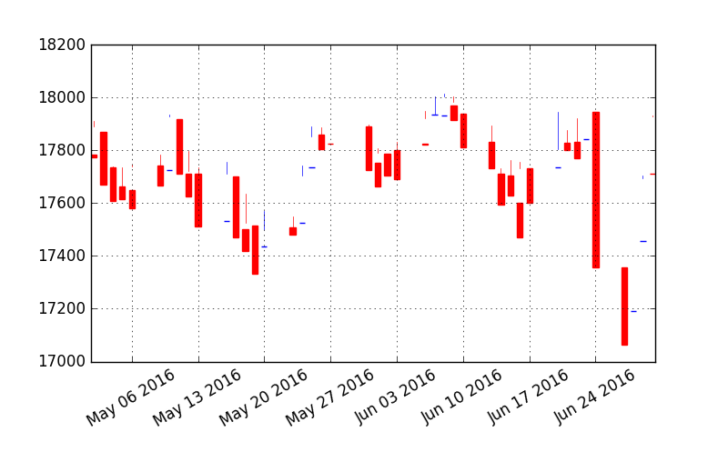
Now if we compare this with R than R seems to be much simpler when it comes to plotting the candlestick charts with quantmod package. Whatever Python and R are 2 powerful data science and machine learning languages that we need to learn. There seems to be a problem with the above candlestick chart. So let’s use the attribute historical_quotes_yahoo_ohlc. This is the correct code. Let’s run the correct code.
#import libraries

import matplotlib.pyplot as plt

import matplotlib.finance as mpf
#import the daily stock quotes from Yahoo Finance
start = (2016, 5, 1)
end = (2016, 6, 30)
quotes = mpf.quotes_historical_yahoo_ohlc(‘^DJI’, start, end)
quotes[:3]
#plot the candlestick chart
fig, ax = plt.subplots(figsize=(8, 5))
fig.subplots_adjust(bottom=0.2)
mpf.candlestick_ohlc(ax, quotes, width=0.6, colorup=’b’, colordown=’r’)
plt.grid(True)
ax.xaxis_date()
# dates on the x-axis
ax.autoscale_view()
plt.setp(plt.gca().get_xticklabels(), rotation=30)
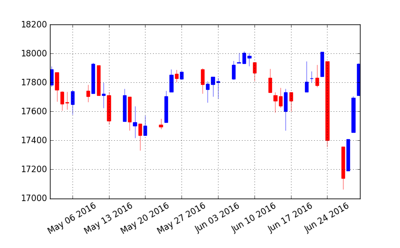
This is the correct candlestick plot of the Dow Jones Index ^DJI daily quotes downloaded from Yahoo Finance.
The point in giving the wrong code in the beginning is for educational purpose. When you are learning how to code you should not be shy of making mistakes. If you are determined and persistent, you will get the code right like us in a few tries. If you read the csv using pandas than you will have to convert the data into a ohlc tuple. The date should first need to be converted to the epoch format that matplotlib.finance can use.