Machine learning and artificial intelligence is the hottest thing right now. There are many hedge funds that are using machine learning in trading now a days. You must have heard and read a lot about quants. Quant are PhDs in Math and Physics. Their job is to develop statistical models that are used by hedge funds to make high alphas. Watch this documentary on Quants. In this post we are going to explore how we can use machine learning in stock trading. If you have been reading my blog then you must have read the last few posts in which I have used python to download stock market data from the web and then do some analysis. Did you read the last post on how to download options data from Yahoo Finance and CBOE.
Python is a powerful modern object oriented language. But in this post we are going to use R. R is a powerful data science and machine learning scripting language. We will be using Microsoft R Open and RStudio. So you should have both these installed. The advantages of Microsoft R Open is that it is much faster than the standard R software that you can download from CRAN. R Open using Intel MKL to use multi-threading that is not possible with standard R. Don’t worry. You can download R Open free just like R. So if you are using windows, you should download R Open and install it on your computer. Did you read the post on how to plot candlestick charts using Python? After reading this post you will realize why R is much better than Python when it comes to financial data analysis. R has a package known as Quantmod. It can very easily convert your stock data into a time series object and plot candlestick as well as bar charts.
Returning to the topic of how to use machine learning in stock trading, the most important thing for a trader is to know the direction of the market. If you can predict market direction with say 80% accuracy, you can keep yourself out of many bad trades. But predicting market direction is a challenging task. There is a lot of noise in the stock market and signal to noise ratio is very low. So finding a profitable signal is a challenge. Challenge is what makes life interesting. So let’s start. Neural networks are powerful tools when it comes to dealing with finding patterns in the data. Algorithmic trading is the name of the game now a days. If you are develop a good algorithmic trading system, you can become rich. Now a days almost something like 80% of the trades that are being placed at Wall Street are being placed by algorithms.You can also watch this documentary on stock market crash that are being caused by rogue algorithms.
Preprocessing The Stock Market Data
We need to download the stock market data. This can be easily done using Quantmod R package. Just type the proper stock ticker symbol and quantmod will be able to fetch the stock data from Yahoo Finance or Google Finance. You can also specify the start and the end dates for the stock data.
> library(quantmod)
> getSymbols("GOOG",src="yahoo")
[1] "GOOG"
> head(GOOG)
           GOOG.Open GOOG.High GOOG.Low GOOG.Close GOOG.Volume GOOG.Adjusted
2007-01-03  466.0008  476.6608 461.1108   467.5908    15470700      233.5618
2007-01-04  469.0008  483.9508 468.3508   483.2608    15834200      241.3890
2007-01-05  482.5008  487.5008 478.1108   487.1908    13795600      243.3521
2007-01-08  487.6908  489.8708 482.2008   483.5808     9544400      241.5489
2007-01-09  485.4508  488.2508 481.2008   485.5008    10803000      242.5079
2007-01-10  484.4308  493.5509 482.0408   489.4608    11981700      244.4859
> tail(GOOG)
           GOOG.Open GOOG.High GOOG.Low GOOG.Close GOOG.Volume GOOG.Adjusted
2017-05-05    933.54   934.900   925.20     927.13     1904700        927.13
2017-05-08    926.12   936.925   925.26     934.30     1321500        934.30
2017-05-09    936.95   937.500   929.53     932.17     1580300        932.17
2017-05-10    931.98   932.000   925.16     928.78     1173900        928.78
2017-05-11    925.32   932.530   923.03     930.60      835000        930.60
2017-05-12    931.53   933.440   927.85     932.22     1038400        932.22
As you can see from the above code, we have download Google stock data. The ticker symbol of Google is GOOG. We just plugged in the ticker symbol in R command and quantmod download 10 years of Google daily stock data in a few seconds. So we have 10 years worth of GOOG daily data. Now we need to do some machine learning on this data that can help us predict future market direction. We want to build a prediction model that can predict whether the market is going to go up, down or simply range. We choose 2% return as a threshold. If the stock moves more than 2% in a day, we call it an up day. If it gives more than -2% return, we have down day. Between 2% and -2%, we say the market is ranging. Watch this documentary on a genius algorithm builder who dared to challenge Wall street.
We will be using a Feedforward Neural Network for doing the machine learning. We will be using the daily close price of GOOG stock. We can also use Adjusted Close. It doesn’t make much difference as long as there has been no stock split. Let’s take a look at GOOG stock data by plotting it over the last 10 years. Take a look at the following chart.
> chartSeries(GOOG, theme="white", TA=NULL)
> goog<- GOOG[,"GOOG.Close"]
As you can see in the chart below, there has been a stock split somewhere in July 2014 when GOOG price was adjusted from $1200 per share to somewhere below $600 per share. You can check the details of the stock split from the internet. Google has made I think 3 stock splits. The last stock split was a bit controversial. Details are available online. You can read about it if you want.
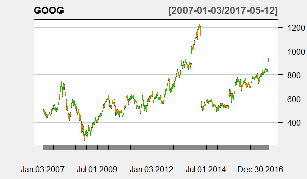
This is very important when you do machine learning. Always make a few plots of the data and see if there are some anomalies that you need to take care of. In this case we need to take into account the stock split that we have just mentioned. This is what we are going to do. We will start our machine learning after August 2014 so that we stay clear of the stock split. As said above since we are staying clear of the stock split, we can use the GOOG daily close.
> goog<- GOOG[,"GOOG.Close"]
> avg10<- rollapply(goog,10,mean)
> avg20<- rollapply(goog,20,mean)
> std10<- rollapply(goog,10,sd)
> std20<- rollapply(goog,20,sd)
> rsi5<- RSI(goog,5,"SMA")
> rsi14<- RSI(goog,14,"SMA")
> macd12269<- MACD(goog,12,26,9,"SMA")
> macd7205<- MACD(goog,7,20,5,"SMA")
Above we calculated the 10 day moving average, 20 day moving average, 10 day standard deviation, 20 day standard deviation, 5 period RSI, 14 period RSI, 12, 26 and MACD and 7, 20 and 5 MACD. Below we calculate the daily return as well as the direction of the stock.
> ret <- Delt(goog)
> direction<- data.frame(matrix(NA,dim(goog)[1],1))
> lagret<- (goog - Lag(goog,20)) / Lag(goog,20)
> direction[lagret> 0.02] <- "Up"
> direction[lagret< -0.02] <- "Down"
> direction[lagret< 0.02 & lagret> -0.02] <- "Range"
> tail(direction)
     matrix.NA..dim.goog..1...1.
2604                          Up
2605                          Up
2606                          Up
2607                          Up
2608                          Up
2609                          Up
> dim(direction)
[1] 2609    1
I have explained before how I calculated the direction. If the return is above 2%, we have an Up day. If we have a return of -2% or more, we have a down day and if the daily return is between 2% and -2%, we have a ranging day. We combine the return with the indicators into one single dataframe below.
> goog<- cbind(goog,avg10,avg20,std10,std20,rsi5,rsi14,macd12269,macd7205,bbands)
Now we choose the dates which we will be dividing the stock daily data into training set, validation set and testing set. The training set will be used to train the neural network model. Validation set will be used for validating the model. Testing set will be used as a final check to see the consistency of the neural network model to make right predictions.
> train_start<- "2015-01-01"
> train_end<- "2015-12-31"
> vali_start<- "2016-01-01"
> vali_end<- "2016-12-31"
> test_start<- "2017-01-01"
As you can see above, we have kept the stock split behind us. We start our machine learning from 2015. So we divide the stock daily data into training set, validation set and testing set below.
> test_end <- "2017-05-12"
> train<- which(index(goog) >= train_start & index(goog) <= train_end)
> validate<- which(index(goog) >= vali_start & index(goog) <= vali_end)
> test<- which(index(goog) >= test_start & index(goog) <= test_end)
Once we divide the data into training, validation and testing date wise, we split the data. R can do it very easily. We just need to know the right command.
> traingoog<- goog[train,]
> valigoog<- goog[validate,]
> testgoog<- goog[test,]
Now we need to normalize the data. Normalization is very important when it comes to training a neural network. Data should be in range 0 and 1.
> trainmean<- apply(traingoog,2,mean)
> trainstd<- apply(traingoog,2,sd)
> trainidn<- (matrix(1,dim(traingoog)[1],dim(traingoog)[2]))
> valiidn<- (matrix(1,dim(valigoog)[1],dim(valigoog)[2]))
> testidn<- (matrix(1,dim(testgoog)[1],dim(testgoog)[2]))
> norm_train<- (traingoog - t(trainmean*t(trainidn))) / t(trainstd*t(trainidn))
> norm_valid<- (valigoog - t(trainmean*t(valiidn))) / t(trainstd*t(valiidn))
> norm_test<- (testgoog - t(trainmean*t(testidn))) / t(trainstd*t(testidn))
> traindir<- direction[train,1]
> validir<- direction[validate,1]
> testdir<- direction[test,1]
Till now we have been doing data preprocessing. Data preprocessing is something very important. We need to do data preprocessing with a lot of care if we want to build a good machine learning model.
Building The Stock Market Neural Network Model
Now comes the machine learning part. We load the nnet package.
> library(nnet)
> model<- nnet(norm_train,class.ind(traindir),size=4,trace=F)
> model
a 15-4-3 network with 79 weights
options were -
> vali_pred<- predict(model,norm_valid)
> head(vali_pred)
                Down Range Up
2016-01-04 0.9999716     0  0
2016-01-05 0.9999714     0  0
2016-01-06 0.9999714     0  0
2016-01-07 0.9999714     0  0
2016-01-08 0.9999714     0  0
2016-01-11 0.9999714     0  0
> vali_pred_class<- data.frame(matrix(NA,dim(vali_pred)[1],1))
> vali_pred_class[vali_pred[,"Down"] > 0.5,1] <- "Down"
> vali_pred_class[vali_pred[,"Range"] > 0.5,1] <- "Range"
> vali_pred_class[vali_pred[,"Up"] > 0.5,1] <- "Up"
> library(caret)
Loading required package: lattice
Loading required package: ggplot2
> library(e1071)
> matrix<- confusionMatrix(vali_pred_class[,1],validir)
This is what we did. We first trained the nnet feedforward neural network with 15 inputs, 4 neuron hidden layer and 3 neuron output layer on the training data. Then we used the trained model to make predictions on the validation data and cross checked it with the actual market direction.
> matrix
Confusion Matrix and Statistics

          Reference
Prediction Down Range Up
     Down    80    26  0
     Range    2    42  6
     Up       0    11 85

Overall Statistics

               Accuracy : 0.8214
                 95% CI : (0.7685, 0.8667)
    No Information Rate : 0.3611
    P-Value [Acc > NIR] : < 2.2e-16

                  Kappa : 0.7308
 Mcnemar's Test P-Value : NA

Statistics by Class:

                     Class: Down Class: Range Class: Up
Sensitivity               0.9756       0.5316    0.9341
Specificity               0.8471       0.9538    0.9317
Pos Pred Value            0.7547       0.8400    0.8854
Neg Pred Value            0.9863       0.8168    0.9615
Prevalence                0.3254       0.3135    0.3611
Detection Rate            0.3175       0.1667    0.3373
Detection Prevalence      0.4206       0.1984    0.3810
Balanced Accuracy         0.9113       0.7427    0.9329
The model accuracy is 82%. Kappa is 0.73. Both model accuracy and model kappa are good. Kappa tells you how much the predictions are based on randomness. Higher kappa values close to 1 indicator less random choice.Now we need to test the model on the testing data. This will give use the feeling how good our machine learning model is on making predictions on unseen data.
> test_pred<- predict(model,norm_test)
> test_pred_class<- data.frame(matrix(NA,dim(test_pred)[1],1))
> test_pred_class[test_pred[,"Down"] > 0.5,1] <- "Down"
> test_pred_class[test_pred[,"Range"] > 0.5,1] <- "Range"
> test_pred_class[test_pred[,"Up"] > 0.5,1] <- "Up"
> test_matrix<- confusionMatrix(test_pred_class[,1],testdir)
Below are the results.
> test_matrix
Confusion Matrix and Statistics

          Reference
Prediction Down Range Up
     Down     5     7  0
     Range    0    29 10
     Up       0     4 36

Overall Statistics

               Accuracy : 0.7692
                 95% CI : (0.6691, 0.8511)
    No Information Rate : 0.5055
    P-Value [Acc > NIR] : 2.157e-07

                  Kappa : 0.6036
 Mcnemar's Test P-Value : NA

Statistics by Class:

                     Class: Down Class: Range Class: Up
Sensitivity              1.00000       0.7250    0.7826
Specificity              0.91860       0.8039    0.9111
Pos Pred Value           0.41667       0.7436    0.9000
Neg Pred Value           1.00000       0.7885    0.8039
Prevalence               0.05495       0.4396    0.5055
Detection Rate           0.05495       0.3187    0.3956
Detection Prevalence     0.13187       0.4286    0.4396
Balanced Accuracy        0.95930       0.7645    0.8469
The predictive accuracy has gone done to 77% with a kappa 0.60. This is just as good as we can get. We can check by improving the neurons in the hidden layer to 10 and see if it makes our model better. You can do that. Let’s backtest the data.
> #bactest the trading strategy
> Signal<- ifelse(test_pred_class =="Up",1,ifelse(test_pred_class =="Down",-1,0))
> ret<- ret[test]
>
> library(PerformanceAnalytics)

Package PerformanceAnalytics (1.4.3541) loaded.
Copyright (c) 2004-2014 Peter Carl and Brian G. Peterson, GPL-2 | GPL-3
http://r-forge.r-project.org/projects/returnanalytics/


Attaching package: ‘PerformanceAnalytics’

The following objects are masked from ‘package:e1071’:

    kurtosis, skewness

The following object is masked from ‘package:graphics’:

    legend

> cost<- 0
> trade_ret<- ret * Lag(Signal)- cost
> cumm_ret<- Return.cumulative(trade_ret)
> annual_ret<- Return.annualized(trade_ret)
> charts.PerformanceSummary(trade_ret)
Below is the plot for this backtesting performance..
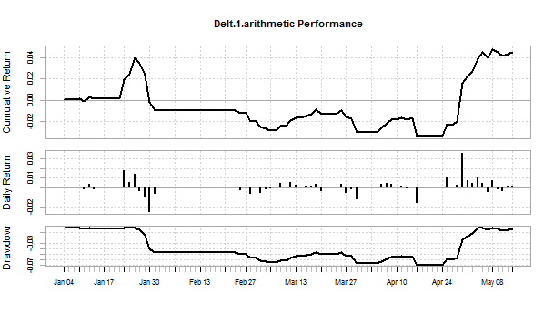
As you can see, this trading strategy is a roller coaster. We need to work on this stock trading strategy more. In the next post I will show you how we are going to improve this stock trading strategy.
I have developed a course on Probability and Statistics for Traders. There are many traders who have no training in probability and statistics. This makes it difficult for them to understand machine learning. Probability and statistics is not difficult. I make everything very easy for you in the course. You can take a look at my course. I take you by hand and teach you everything that you need to know. My course is focused on financial markets and how to apply probability and statistics to your trading.
As said in the start of this post, algorithmic trading is now the name of the game. Days of manual trading are coming to an end. Did you notice one thing? Traditional indicators like MACD, RSI, Stochastic, CCI etc. are now working any more. Candlestick patterns are most of the time giving bad trades one after another. Why? Have you pondered on this? Answer is simple. Traditional technical analysis was developed in 1950s to 1980s. Today it doesn’t work because we have much better predictive models that are being used by hedge funds and the big banks. Using modern predictive models can improve your trading a lot. I have provided you with an example. I used a simple feedforward neural network. Trained it and then used it to make predictions on a particular stock. Today a revolution is taking place in artificial intelligence. You should learn how to apply artificial intelligence to your trading.